The Global Self-consistent, Hierarchical, High-resolution Geography (GSHHG) database is an amalgamation of two public domain databases by Paul Wessel (SOEST, University of Hawaii, Honolulu, HI) and Walter Smith (NOAA Laboratory for Satellite Altimetry, Silver Spring, MD) (Wessel and Smith 1996). The format of the GSHHG changed and therefore the recipes contained in MRES and MDRES have to be modified.
The GSHHG database consists of the older GSHHS shoreline database (Soluri and Woodson 1990, Wessel and Smith 1996), which is a shoreline database, with the poor quality Antarctica data replaced by the more accurate data from Bohlander and Scambos (2007), and with rivers and borders taken from the CIA World Data Bank II (WDBII) (Gorny 1977). The GSHHG data can be downloaded from the SOEST server in three different formats: Generic Mapping Tools (GMT) files, ESRI shapefiles, or native binary files, and in a wide range of spatial resolutions. This example uses version 2.3.6 of the native binary file gshhg-bin-2.3.6.zip. We use the MATLAB unzip function to decompress this file
clear, clc, close all
unzip('gshhg-bin-2.3.6.zip')
which creates files containing the shorelines (gshhs), borders (wdb_borders) and rivers (wdb_rivers), each at different resolutions ranging from f (full resolution, 95.8 MB large) to c (crude resolution, 183 kb large), as explained on Paul Wessel’s SOEST webpage. As an example we import the high-resolution shoreline data set from file gshhs_h.b using
S = gshhs('gshhs_h.b');
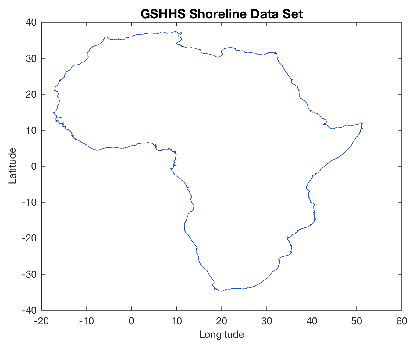
We obtain a structure array S which includes the longitude/latitude coordinates of the shoreline segments together with various other types of information. The elements of S contain the shorelines of the continents and islands, for example S(2) contains the longitude/latitude coordinates of Africa. We can extract the shoreline coordinates by typing
data(:,1) = S(2).Lon;
data(:,2) = S(2).Lat;
We save the longitude/latitude coordinates in an ASCII file using
save coastline_data.txt data -ascii
and load it after clearing the workspace using
clear

data = load('coastline_data.txt');
There are different ways of displaying the data. As an example, we can use the line command to create a line plot, after having defined the figure and axes properties, as follows:
figure1 = figure('Color',[1 1 1]);
axes1 = axes('Box','on',...
     'DataAspectRatio',[1 1 1]);
line1 = line(data(:,1),data(:,2),...
     'Color',[0 0 0]);
xlabel1 = xlabel('Longitude');
ylabel1 = ylabel('Latitude');
More advanced plotting functions are contained in the Mapping Toolbox, which allows alternative versions of this plot to be generated:
axesm('MapProjection','lambert', ...
    'MapLatLimit',[0 15], ...
    'MapLonLimit',[35 55], ...
    'Frame','on', ...
    'MeridianLabel','on', ...
    'ParallelLabel','on');
plotm(data(:,2),data(:,1),'k');
Note that the input for plotm is given in the order longitude, followed by the latitude, i.e., the second column of the data matrix is entered first. In contrast, the function plot requires an xy input, i.e., the first column is entered first. The function axesm defines the map’s axes and sets various map properties such as the map projection, the map limits and the axis labels.
References
Bohlander, J, Scambos T (2007) Antarctic coastlines and grounding line derived from MODIS Mosaic of Antarctica (MOA). National Snow and Ice Data Center, Boulder, Colorado
Soluri EA, Woodson VA (1990), World Vector Shoreline. International Hydrographic Review LXVII(1):27–35
Gorny AJ (1977) World Data Bank II General User Guide Rep. PB 271869. Central Intelligence Agency, Washington DC
Wessel P, Smith WHF (1996) A Global Self-consistent, Hierarchical, High-resolution Shoreline Database. Journal of Geophysical Research 101 B4: 8741-8743.