
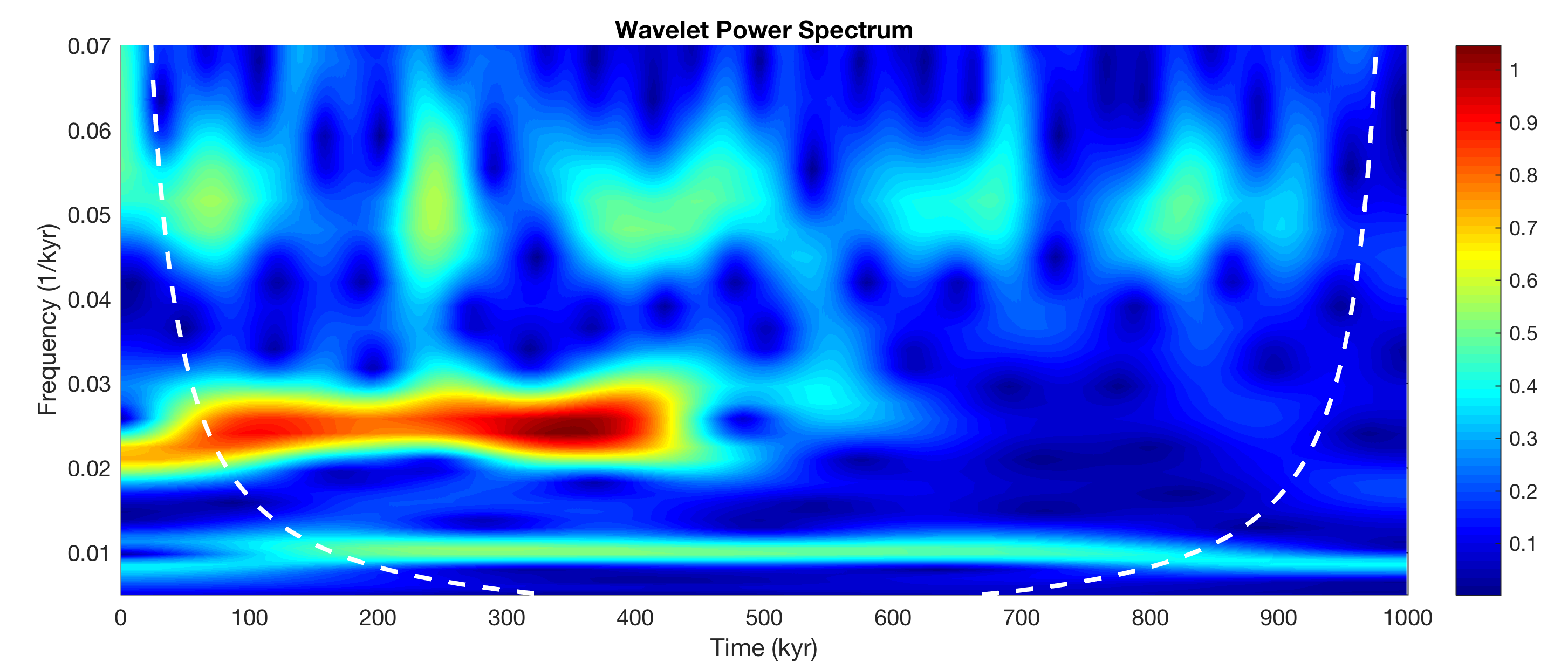
After having talked to MathWorks Support I managed to display the cone of influence coi together with the wavelet transform wt. The cone of influence marks the area were edge effects occur in the continuous 1D wavelet transform.
The script is the same as in the previous post about the new function cwt. We first load data from series3, interpolate the data upon an evenly spaced time vector, detrend the data and calculate the wavelet transform using cwt.
clear, clc
series3 = load('series3.txt');
t = 0 : 3 : 1000;
series3L = interp1(series3(:,1),...
     series3(:,2),t,'linear','extrap');
series3L = detrend(series3L);
[wt,f,coi] = cwt(series3L,1/3);
According to the philosophy of MRES, we try to reproduce algorithms for data analysis by simple means. In this case it is about understanding the graphical output of ctw and trying to reproduce it. According to the documentation the data format of coi is either a array of doubles or an array of duration objects. Using frequencies instead of periods as y-axes we can use simply use line(t,coi) to display the cone of influence by typing
figure('Position',[100 300 800 300],...
    'Color',[1 1 1]);
pcolor(t,f,abs(wt)), shading interp
hold on
line(t,coi,'Color','w',...
    'LineStyle','--',...
    'LineWidth',2)
xlabel('Time (kyr)')
ylabel('Frequency (1/kyr)')
title('Wavelet Power Spectrum')
set(gcf,'Colormap',jet)
set(gca,'XLim',[0 1000],...
 'YLim',[0.005 0.07],...
 'XGrid','On',...
 'YGrid','On')
colorbar