
What is a good sample size? How many replicate measurements do we need to make inferences about a population from the sample? There are scientific articles on this subject, such as the one by H.W. Austin (1983), of which the title of the blog post is borrowed. There is no universal answer to this question. It depends very much on the studied phenomenon and the requirements on the results. Here is a nice example of how MATLAB helps to get a sense of the relationship between sample size and quality of the result.
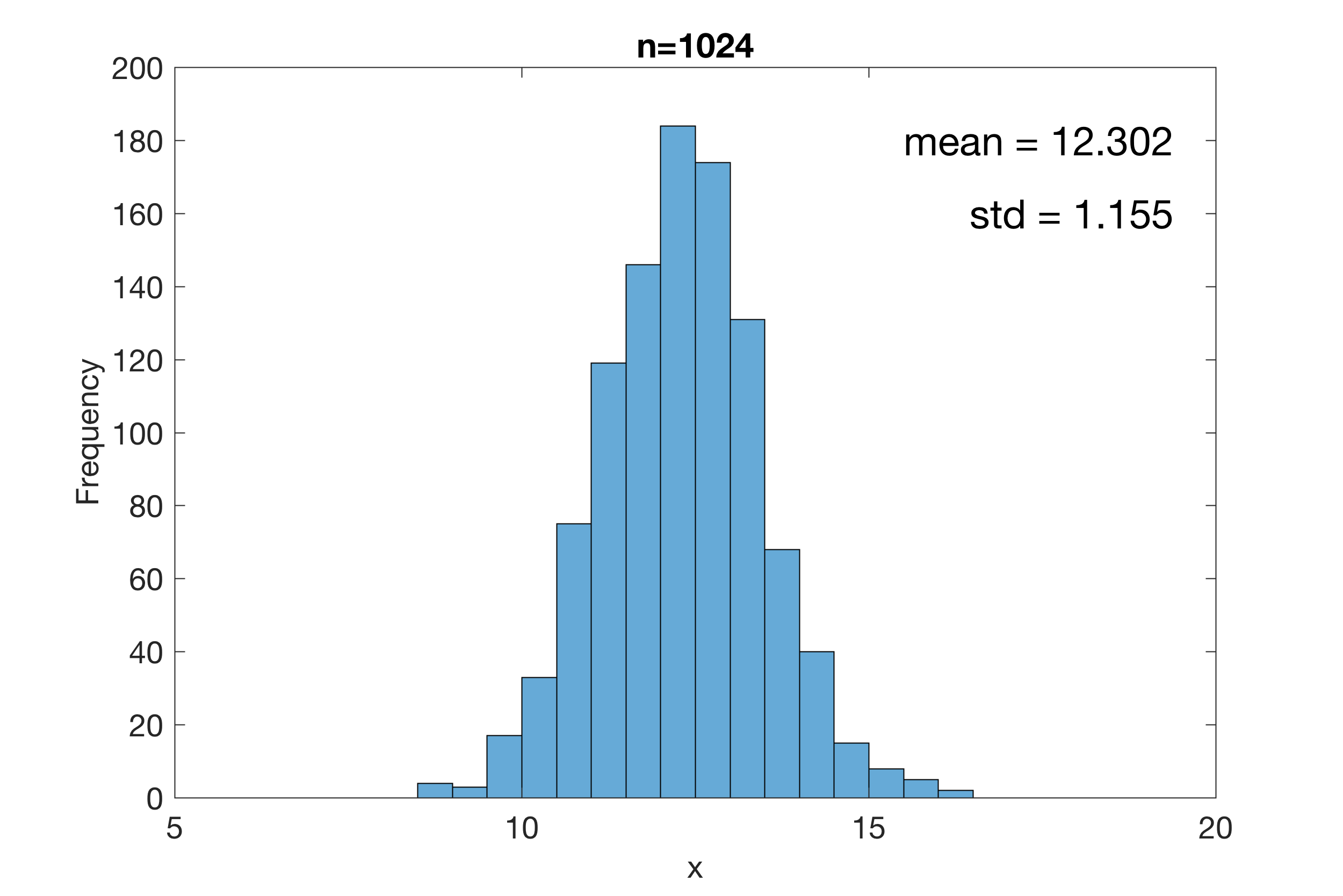
We look at one of the simplest examples to show the relationship between sample size and the precision of the parameters to be estimated. We use a random number generator to generate n replicate measurements from a Gaussian distribution with a population mean of 12.34 and a population standard deviation of 1.16. Since n<∞ our mean and standard deviation calculated from the sample are different from these two values, depending on the sample size n.
We first define an array n, which contains the sample sizes from 2 to 2^25=3,355,4432.
clear
n = 2.^[1:25];
Next we prepare the video file amovie_1.avi using VideoWriter, define the frame rate of 1 frame per second and video quality of 100%. We then check the parameter settings and open the file.
v = VideoWriter('amovie_1.avi');
v.FrameRate = 5;
v.Quality = 100;
open(v);
Then we run an animated display of a histogram display of the data corg and record the video by typing
for i = 1 : length(n)

close all
rng(0)
corg = 12.34 + 1.16 * randn(n(i),1);

figure(...
    'Position',[200 200 600 400],...
    'Color',[1 1 1]);
h1 = histogram(corg);
set(gca,'Box','on',...
    'Units','Centimeters',...
    'LineWidth',0.5,...
    'FontName','Helvetica',...
    'FontSize',14,...
    'XLim',[5 20]);
h2 = xlabel('x');
set(h2,'FontName','Helvetica',...
    'FontSize',14);
h3 = ylabel('Frequency');
set(h3,'FontName','Helvetica',...
    'FontSize',14);
titlestring = ['n=',num2str(n(i))];
title(titlestring)
textstring1 = [...
     'mean = ',num2str(mean(corg),'%2.3f')];
text(0.97*20,max(get(gca,'YLim'))*0.9,...
    textstring1,...
    'HorizontalAlignment','right',...
    'FontSize',18)
textstring2 = [...
    'std = ',num2str(std(corg),'%2.3f')];
text(0.97*20,max(get(gca,'YLim'))*0.8,...
    textstring2,...
    'HorizontalAlignment','right',...
    'FontSize',18)

mmean(i) = mean(corg);
mstd(i) = std(corg);

M = getframe(gcf);
writeVideo(v,M);

end
close(v);
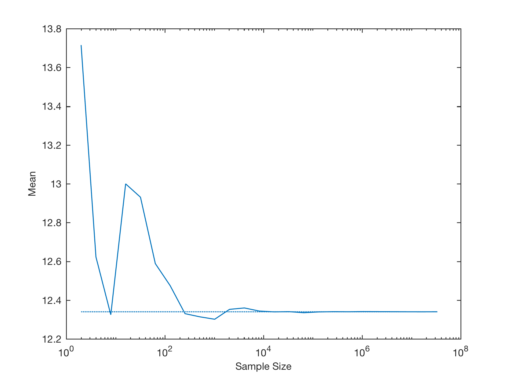
The histograms show the sample mean and sample standard deviation in the upper right corner. We can also display the sample mean over the sample size (on a log scale) by typing
figure(...
    'Position',[200 200 400 300],...
    'Color',[1 1 1]);
axes(...
    'Box','on',...
    'XScale','log',...
    'LineWidth',0.6,...
    'FontName','Helvetica',...
    'FontSize',8); hold on
line(n,mmean,...
    'Color',[0 0.4453 0.7383],...
    'LineWidth',0.75);
line(n,12.34*ones(size(n)),...
    'Color',[0 0.4453 0.7383],...
    'LineWidth',0.75,...
    'LineStyle',':');
xlabel(...
    'Sample Size',...
    'FontName','Helvetica',...
    'FontSize',8);
ylabel(...
    'Mean',...
    'FontName','Helvetica',...
    'FontSize',8);
And finally we display the sample standard deviation over the sample size (on a log scale) by typing
figure(...
    'Position',[200 200 400 300],...
    'Color',[1 1 1]);
axes(...
    'Box','on',...
    'XScale','log',...
    'LineWidth',0.6,...
    'FontName','Helvetica',...
    'FontSize',8); hold on
line(n,mstd,...
    'Color',[0.8477 0.3242 0.0977],...
    'LineWidth',0.75);
line(n,1.16*ones(size(n)),...
    'Color',[0.8477 0.3242 0.0977],...
    'LineWidth',0.75,...
    'LineStyle',':');
xlabel(...
    'Sample Size',...
    'FontName','Helvetica',...
    'FontSize',8);
ylabel(...
    'Standard Deviation',...
    'FontName','Helvetica',...
    'FontSize',8);
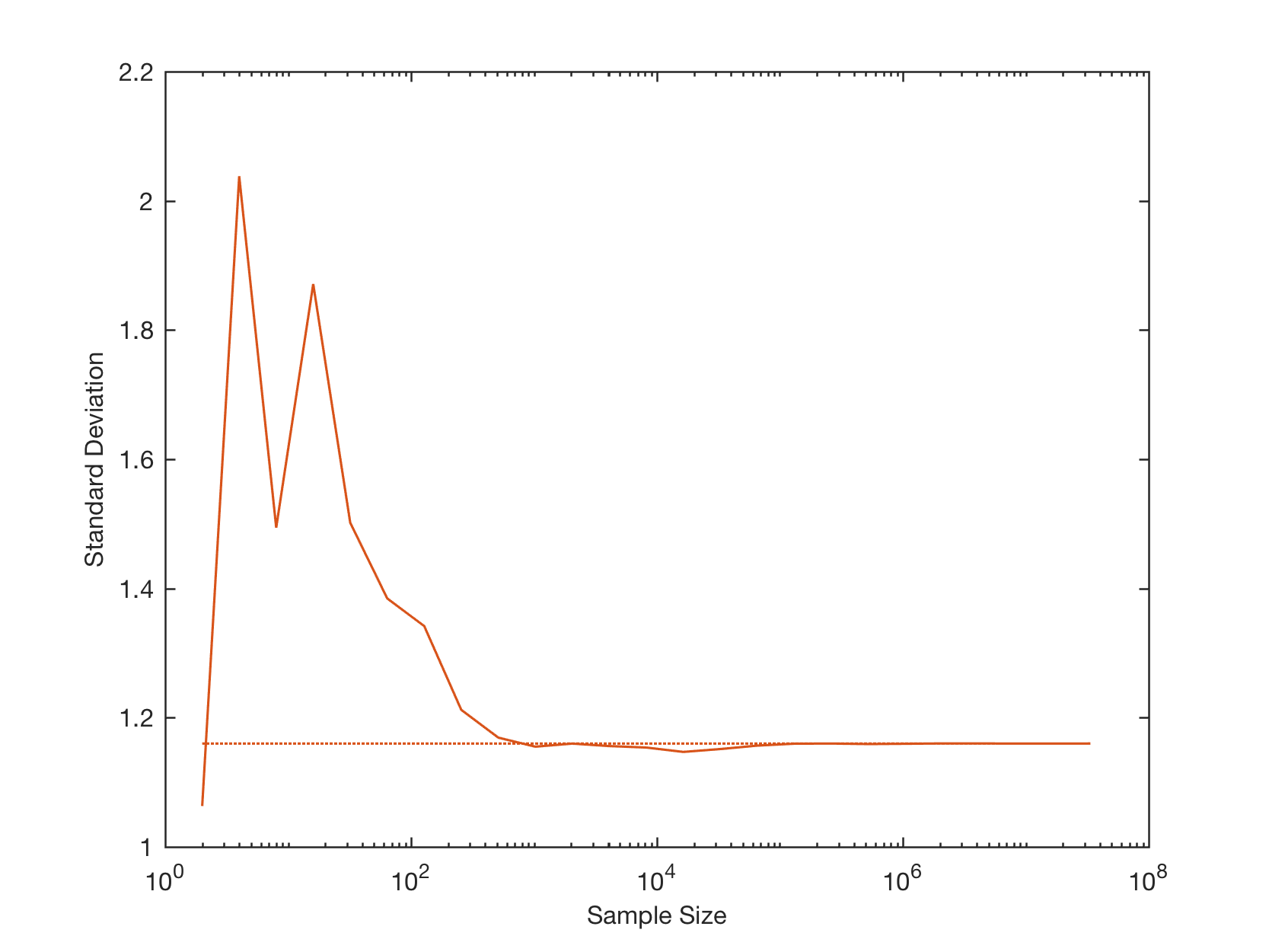
In both graphics, the horizontal dotted lines depict the statistical parameters mean and standard deviation of the population, as we defined it when we used the random number generator. As you can see we need a sample size of about 10^3 or 1,000 to get estimates of the mean and the standard deviation close to the true values.
The MATLAB script above also generates an animation which is shown below. Comments on this are, as always, very welcome via email!
References
Austin, H.W. (1983) Sample Size: How Many is Enough? Quality and Quantity, 17, 239-245.