
In MATLAB R2016b, the function to calculate a continuous 1D wavelet transform has been replaced by a new function, unfortunately with the same name. Here is a great example why I think that this blog is very useful: Here I can let you know how I would modify the script of Chapter 5.8 of MRES and ask for your comments on it, long before the 5th edition of MRES will be published.
I use the same synthetic data stored in the file series3.txt as an example. As before, you first have to interpolate your data to an evenly spaced time vector t, using the minimum and maximum values of your original time axes and a sampling interval close to the mean sampling interval of your data, which is 3.0030 in my synthetic example.
clear, clc
series3 = load('series3.txt');
mean(diff(series3(:,1)))

t = 0 : 3 : 1000;
series3L = interp1(series3(:,1),...
   series3(:,2),t,'linear','extrap');
If your time series has a trend please detrend it before running the Wavelet analysis:
series3L = detrend(series3L);
Then you use cwt with the data series series3L and the inverse of your sampling interval. In our example, the sampling interval is 3, therefore the sampling frequency is 1/3. The output is the wavelet transform wt, the frequencies f and the cone of influence coi to mark the area were edge effects occur in the CWT. This is the new cwt function introduced with MATLAB R2016b. It uses an DFT-based algorithm, similar to the one introduced by Torrence and Compo (Here is a link to their classic Wavelet webpage, also cited in my textbook) and which was already used by the old function cwtft which is no longer supported, similar to the old version of cwt.
The advantage of the new cwt function that it provides defaults, different from the old version, allowing to run a wavelet analysis without caring too much about the settings. According to the documentation of the function, the cwt is obtained using the analytic Morse wavelet with the symmetry parameter (gamma) equal to 3 and the time-bandwidth product equal to 60. The function cwt uses 10 voices per octave. Here is some background information about the case by The MathWorks Inc. about the change.
[wt,f,coi] = cwt(series3L,1/3);
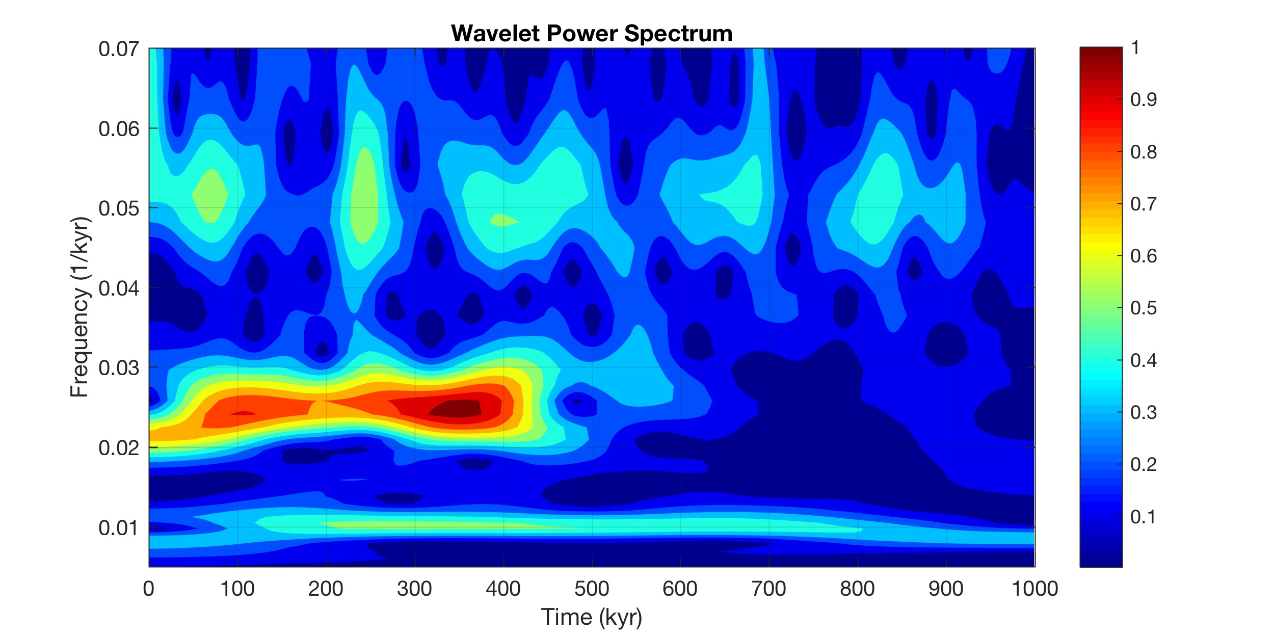
Now we display the wavelet power spectrum. You can change the limits of the axes, the colormap and many other things. I did not yet successfully plot the cone of influence here. You can see cycles with frequencies of 0.01/kyr (corresponding to a period of 100 kyr), 0.025 (40 kyr) and 0.05 (20 kyr). The great thing about Wavelets is that it displays an evolutionary spectrum, i.e. the appearance and disappearance of cycles through time.
figure('Position',[100 300 800 300],...
   'Color',[1 1 1]);
contour(t,f,abs(wt),...
   'LineStyle','none',...
   'LineColor',[0 0 0],...
   'Fill','on')
xlabel('Time (kyr)')
ylabel('Frequency (1/kyr)')
title('Wavelet Power Spectrum')
set(gcf,'Colormap',jet)
set(gca,'XLim',[0 1000],...
   'YLim',[0.005 0.07],...
   'XGrid','On',...
   'YGrid','On')
colorbar
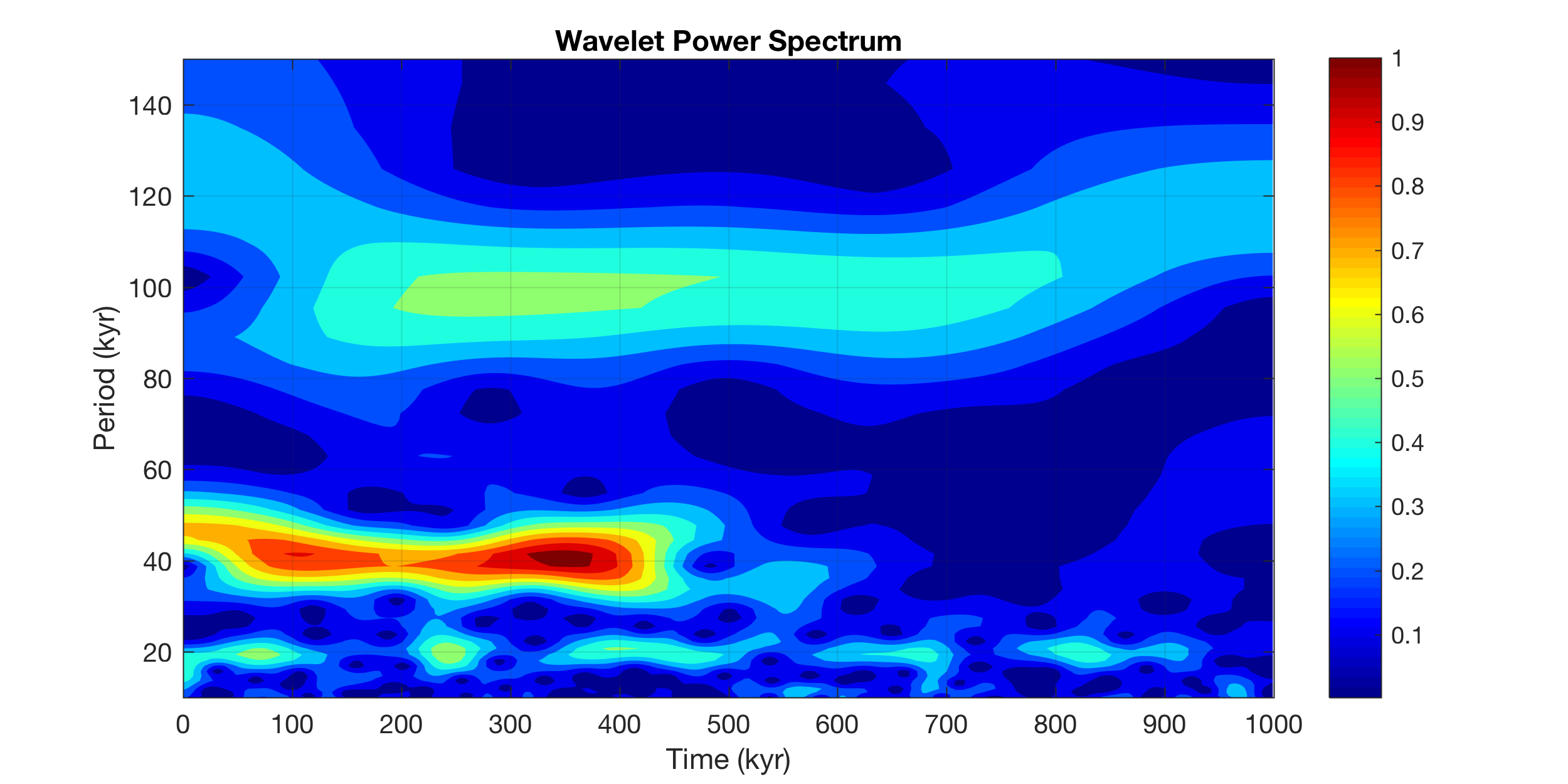
The same plot with periods instead of frequencies on the y-axis. You can see cycles with a period of 100 kyr, 40 kyr and 20 kyr.
figure('Position',[100 300 800 300],...
   'Color',[1 1 1]);
contour(t,1./f,abs(wt),...
   'LineStyle','none',...
   'LineColor',[0 0 0],...
   'Fill','on')
xlabel('Time (kyr)')
ylabel('Period (kyr)')
title('Wavelet Power Spectrum')
set(gcf,'Colormap',jet)
set(gca,'XLim',[0 1000],...
   'YLim',[10 150],...
   'XGrid','On',...
   'YGrid','On')
colorbar
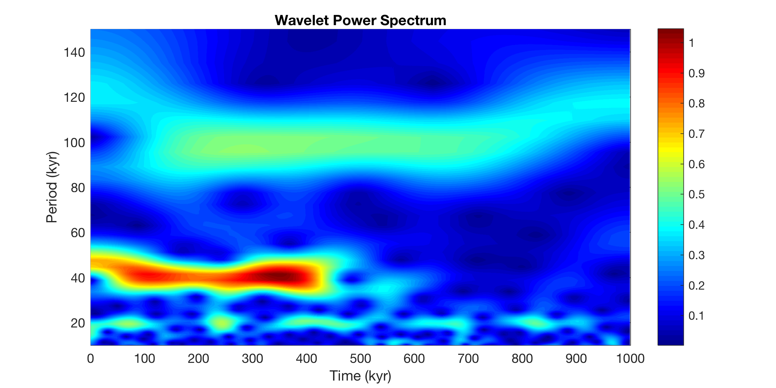
The same plot using pcolor instead of contour.
figure('Position',[100 300 800 300],...
   'Color',[1 1 1]);
pcolor(t,1./f,abs(wt)), shading interp
xlabel('Time (kyr)')
ylabel('Period (kyr)')
title('Wavelet Power Spectrum')
set(gcf,'Colormap',jet)
set(gca,'XLim',[0 1000],...
   'YLim',[10 150])
colorbar
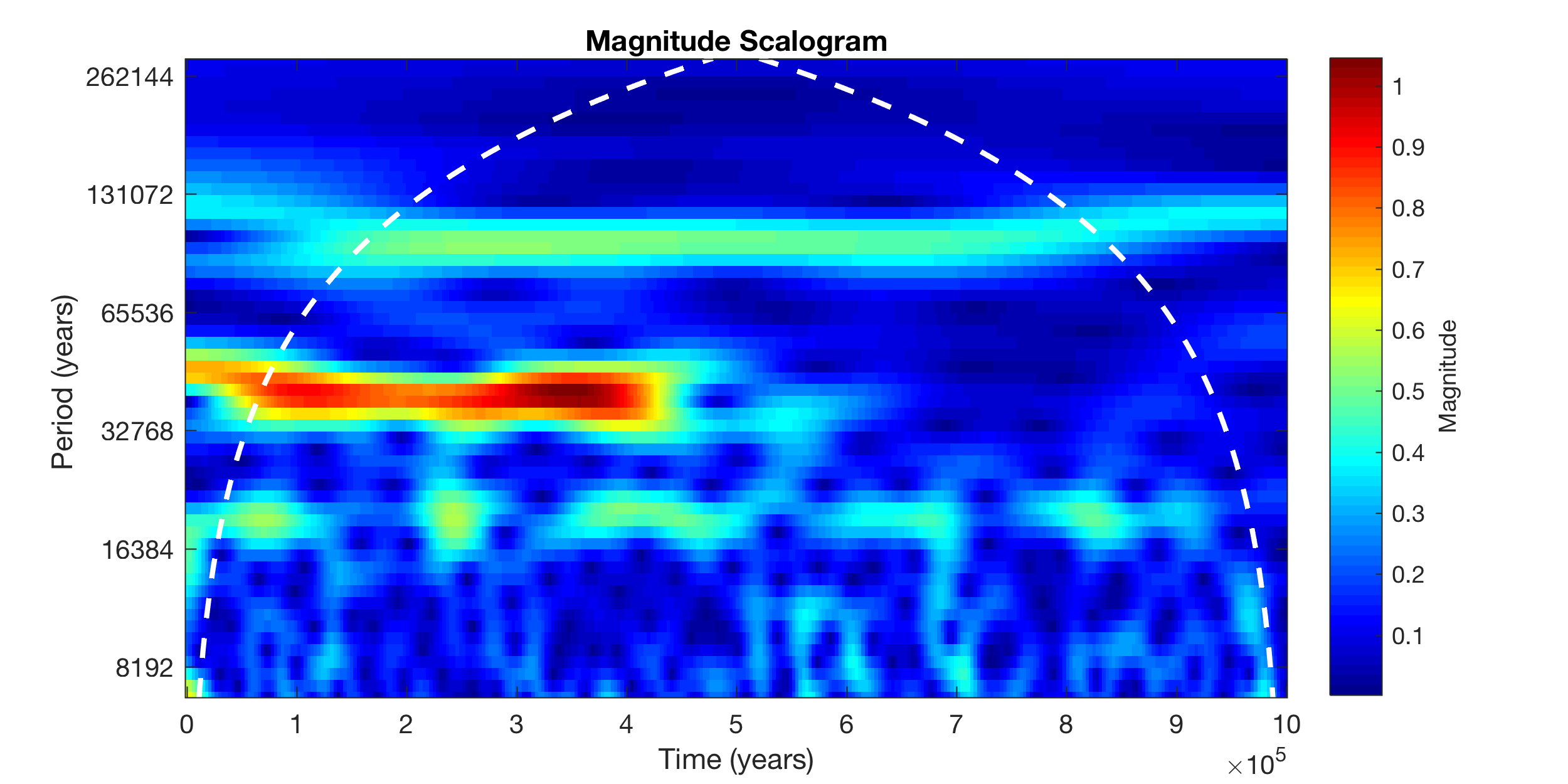
Alternatively, we can use the graphical output of the function cwt. It is a bit tricky to change the display of the graphics. Unfortunately changing the axes limits is tricky because the axes are independent from the colorful display of the wavelet transform. Browsing the code of cwt reveals that it actually uses imagesc to create the pseudocolor plot and then create an independent axis system on top of that. I will keep trying, the numbers on the y-axis really look bad. Typing doc ctw in the Command Window shows that the developers obviously do not care about the tick labels.
figure('Position',[100 300 800 300],...
   'Color',[1 1 1]);
cwt(series3L,years(3000))
colormap(jet)
Do you like the new cwt function? Here is the a zipped archive of the MATLAB live script, the classic script and the PDF version of the live script, together with the synthetic data file. Commands via email are, as always, very welcome. Please note that there is an update of this post.