Cluster Analysis with MATLAB – MATLAB and Python Recipes for Earth Sciences

Cluster analysis creates groups of objects that are very similar to one another compared with other individual objects or groups of objects. The aim of the method is to gain insights into the structure of a data set without predefining categories and therefore cluster analysis is a method of unsupervised learning.

In earth sciences, the method is used to group volcanic ash samples in order to assign them to individual volcanic eruptions with the aim of creating a tephronology for a region (e.g., Hermanns et al. 2000). Another example is the classification of pollen spectra with the aim of defining pollen zones with similar vegetation in the past (e.g. Vincent et al. 2010). As a third example, clustering is used in remote sensing to group pixel with similar spectral signature in order to classify and map different types of soil, rock or vegetation (e.g., Lein 2012).

Numerous methods exist in cluster analysis, each of which use a different approach to create clusters. The popular hiercharchical clustering first calculates the similarity (or dissimilarity) of objects and then builds a tree of clusters merging or splitting objects depending on the similarity (or dissimilarity), commonly displayed in a dendrogram. K-means clustering groups the objects into K groups so that the sum of the squared deviations of all objects from the respective group center is minimal. Spectral clustering first represents the objects in a similarity graph, where the objects are the vertices of the graph and the edges represent the similarity between the objects. Then, the spectrum (the eigenvalues) of the similarity matrix is calculated to transform the data into a lower-dimensional space in which clusters can be more easily identified. Finally, a standard method such as K-means clustering is used to actually group the objects. The last method, k-nearest neigbor classification and clustering, which is strictly speaking not clustering, nor is it a method of unsupervised classification, finds groups of objects with many close neigbors inside the group, but few connections to objects outside.

The following introduction offers a very brief insight into this extensive topic. It presents the three most popular methods of cluster analysis in the earth sciences, as well as a fourth method that can be used to calculate clusters, but with the aid of a training dataset and is therefore a method of supervised machine learning. The MATLAB examples below use is the synthetic data set from Ch. 9.5 of the MRES book, where only one method of clustering, namely hierarchical clustering, is presented. Although K-means clustering and k-nearest neighbor clustering are also briefly mentioned in Ch. 9.5, they are not discussed in detail and are not explained using an example. Spectral clustering, a method for generating clusters that is related to principal component analysis, is not covered in the book. Spectral clustering, which, like principal component analysis from Ch. 9.2 of the MRES book, uses eigenvectors and eigenvalues to reduce the dimensionality of the data set, is not covered in the book.

Hierarchical Clustering

Hierarchical clustering creates groups of objects that are very similar to one another compared with other individual objects or groups of objects. This method first computes the similarity or (alternatively) the dissimilarity (or distance) between all pairs of objects. It then ranks the groups according to their similarity (or distance from one another) before finally creating a hierarchical tree, which is visualized as a dendrogram. A threshold distance is applied to define the number of clusters. Numerous methods exist for calculating the similarity or (alternatively) the dissimilarity (or distance) between two data vectors. Let us define two data sets consisting of multiple measurements from the same object. These data can be described by vectors:

The most popular measure of dissimilarity (or distance) between any two sample vectors is the Euclidean distance. This is simply the shortest distance between the two points that describe two measurements in the multivariate space:

The Euclidean distance is certainly the most intuitive measure of dissimilarity. However, in heterogeneous data sets consisting of a number of different types of variables, a better alternative would be the Manhattan (or city block) distance. In the city of Manhattan, it is necessary to follow perpendicular avenues rather than crossing blocks diagonally. The Manhattan distance is therefore the sum of all differences:

Measures of similarity include the correlation similarity coefficient. This measure uses Pearson’s linear product–moment correlation coefficient to compute the similarity between two objects:

The measure is used if a researcher is interested in the ratios between the variables measured on the objects. However, Pearson’s correlation coefficient is highly sensitive to outliers and should be used with care. An alternative measure of similarity is the inner product similarity index. Normalizing the length of the data vectors to a value of one and computing their inner product yields another important similarity index that is often used in transfer function applications. In this example, a set of modern flora or fauna assemblages with known environmental preferences is compared with a fossil sample in order to reconstruct past environmental conditions:

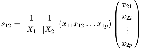
The inner product similarity varies between 0 and 1. A zero value suggests no similarity and a value of one suggests maximum similarity.

The second step in performing a cluster analysis is to rank the groups by their similarity and to build a hierarchical tree, which is visualized as a dendrogram. Most clustering algorithms simply link the two objects with the highest level of similarity or dissimilarity (or distance) (e.g. Hermanns et al. 2000). In the following steps, the most similar pairs of objects or clusters are linked iteratively. A variant of hierarchical clustering, (stratigraphically) constrained clustering, is used in palynology, where pollen samples are only grouped if they directly follow each other in a stratigraphic sequence or in a sediment core (e.g. Vincens et al. 2010). In both examples, the difference between clusters (each of which is made up of groups of objects) is described in different ways depending on the type of data and the application.

As an exercise in performing hierarchical clusterering, the sediment data stored in sediment_3.txt are loaded. This data set includes the percentages of various minerals contained in sediment samples. The sediments are sourced from three rock types: (1) a magmatic rock containing amphibole, pyroxene, and plagioclase; (2) a hydrothermal vein characterized by the presence of fluorite, sphalerite, and galena as well as by some feldspars (i.e., plagioclase and potassium feldspars) and quartz; and (3) a sandstone unit containing feldspars, quartz, and clay minerals. Ten samples were taken from various levels in this sedimentary sequence, and each sample contains varying proportions of these minerals. Therefore, the rows in data correspond to the samples, the columns correspond to the variables.

clear, clc, close all
data = load('sediments_3.txt');

We then create decent colors for the graphics.

colors = [
   0      0.4470 0.7410
   0.8500 0.3250 0.0980
   0.9290 0.6940 0.1250
   0.4940 0.1840 0.5560
   0.4660 0.6740 0.1880
   0.3010 0.7450 0.9330
];

First, the distances between pairs of samples can be computed. The function pdist provides many different measures of distance, such as the Euclidean or Manhattan (or city block) distance. We use the default setting, which is the Euclidean distance:

Y = pdist(data);

The function pdist returns a vector Y containing the distances between each pair of observations in the original data matrix. We can visualize the distances in a heatmap:

figure('Position',[50 900 600 400])
heatmap(squareform(Y));
title('Euclidean Distance Between Pairs of Samples')
xlabel('First sample no.')
ylabel('Second sample no.')

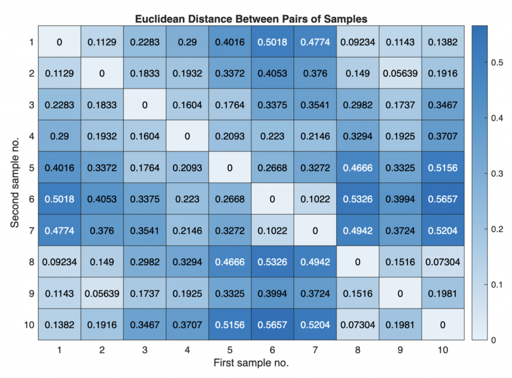
The function squareform converts Y into a symmetric, square format such that the elements (i,j) of the matrix denote the distance between the i and j objects in the original data. We next rank and link the samples with respect to their separation distances to create an agglomerative hierarchical cluster tree using linkage:

Z = linkage(Y)

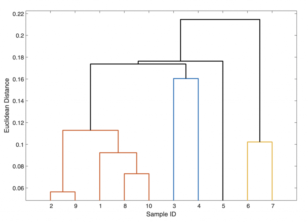
In this 3-column array Z, each row identifies a link. The first two columns identify the objects (or samples) that have been linked, while the third column contains the separation distance between these two objects. The first row (link) between objects (or samples) 1 and 2 has the smallest distance, which corresponds to the greatest similarity. In our example, samples 2 and 9 have the smallest separation distance (i.e., 0.0564) and are therefore grouped together and given the label 11 (i.e., the next-available index higher than the highest sample index of 10). Next, samples 8 and 10 are grouped into 12 since they have the second-smallest separation difference (i.e., 0.0730). The next row shows that the new group 12 is then grouped with sample 1 (i.e., the two items have a separation difference of 0.0923), and so forth. Finally, we visualize the hierarchical clusters as a dendrogram:

figure('Position',[50 800 600 400])
h1 = dendrogram(Z);
xlabel('Sample ID')
ylabel('Euclidean Distance')
box on

set(h1,'LineWidth',1.5,...
   'Color',[0 0 0])

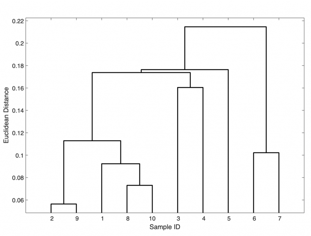
The dendrogram shows clear groups consisting of (a) samples 1, 2, 8, 9, and 10 (i.e., the magmatic source rocks); (b) samples 3, 4, and 5 (i.e., the magmatic dyke containing ore minerals); and (c) samples 6 and 7 (i.e., the sandstone unit). A variant of the dendrogram is the one using threshold of an Euclidean distance of 0.12:

figure('Position',[50 700 600 400])
h2 = dendrogram(Z,'ColorThreshold',0.17);
xlabel('Sample ID')
ylabel('Euclidean Distance')
box on
set(h2,'LineWidth',1.5)
for i = 1 : size(h2,1)
   if get(h2(i),'Color')==[1 0 0]
       set(h2(i),'Color',colors(1,:))
   elseif get(h2(i),'Color')==[0 1 0]
       set(h2(i),'Color',colors(2,:))
   elseif get(h2(i),'Color')==[0 0 1]
       set(h2(i),'Color',colors(3,:))
   end
end

One way of testing the validity of our clustering result is by using the cophenetic correlation coefficient,

cophenet(Z,Y)

which is 0.7579 in our example. The result is convincing since the closer this coefficient is to one, the better the cluster solution is.

K-Means Clustering

Another very popular method of clustering is K-means clustering. Here, the user first defines the number K of clusters. The algorithm then calculates the centroids, such as the multivariate means, of any K initial clusters. The algorithm then iteratively computes improved centroids with the aim of minimizing the sum of the squared distances of the objects from the K centroids. The same distance measures are used here as for hierarchical clustering, such as the Euclidean distance or cityblock distance. Since K-means clustering uses the distance between the centroids as a measure of the difference between the groups, the method is used if the data suggest that there is a central value surrounded by random noise. A disadvantage of the method is that the user has to specify the number of centroids.

As an exercise in performing hierarchical clusterering, again the sediment data stored in sediment_3.txt are loaded. This data set includes the percentages of various minerals contained in sediment samples. The sediments are sourced from three rock types: (1) a magmatic rock containing amphibole, pyroxene, and plagioclase; (2) a hydrothermal vein characterized by the presence of fluorite, sphalerite, and galena as well as by some feldspars (i.e., plagioclase and potassium feldspars) and quartz; and (3) a sandstone unit containing feldspars, quartz, and clay minerals. Ten samples were taken from various levels in this sedimentary sequence, and each sample contains varying proportions of these minerals. Therefore, the rows in data correspond to the samples, the columns correspond to the variables.

clear, clc, close all
data = load('sediments_3.txt');

We then create decent colors for the graphics.

colors = [
    0      0.4470 0.7410
    0.8500 0.3250 0.0980
    0.9290 0.6940 0.1250
    0.4940 0.1840 0.5560
    0.4660 0.6740 0.1880
    0.3010 0.7450 0.9330
];

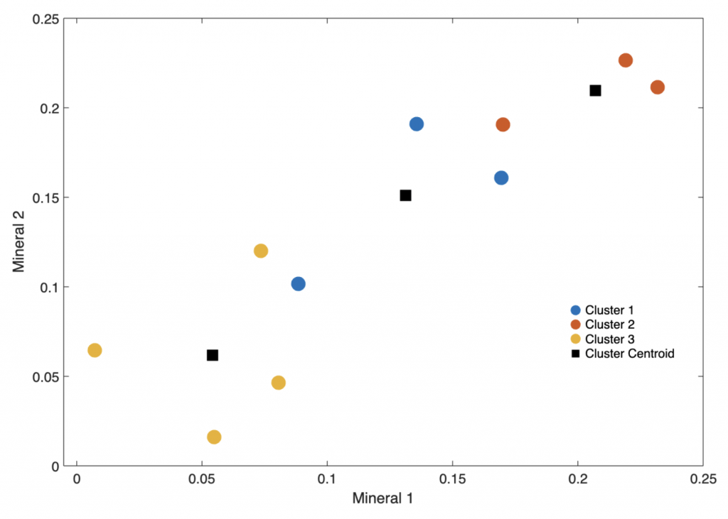
The function kmeans chooses random initial cluster centroid positions to choose initial cluster centroid positions, sometimes known as seeds. Reseting the random number generator with rng(0) makes sure that we always get the same result.

rng(0)
[idx,C] = kmeans(data,3)

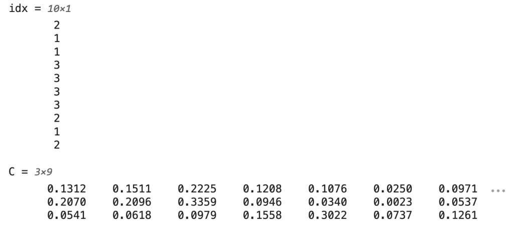
Display data in a 2D plot of Minerals 1 and 2, i.e. the first and second column of the data set. The data points are colored according to their respective clusters together with the cluster centroids.

figure('Position',[50 600 600 400])
h3 = gscatter(data(:,1),data(:,2),idx);
hold on
plot(C(:,1),C(:,2),...
   'LineStyle','None',...
   'Marker','Square',...
   'MarkerSize',10,...
   'MarkerFaceColor',[0 0 0],...
  'Color',[0 0 0])
xlabel('Mineral 1')
ylabel('Mineral 2')
for i = 1 : size(h3,1)
   set(h3(i),'Marker','o',...
      'MarkerSize',10,...
      'MarkerFaceColor',colors(i,:))
end
legend('Cluster 1','Cluster 2',...
   'Cluster 3','Cluster Centroid',...
   'Box','Off')
hold off

Spectral Clustering

Spectral clustering uses a graph-based algorithm to find k shaped clusters in the data set. First, a similarity graph is created in which the objects represent the vertices of the graph, while the edges represent the similarity between objects. The relationships between the nodes and edges of a graph are represented by the Laplace matrix. The eigenvalues of the Laplace matrix, also known as the spectrum of the similarity matrix, can be used to transform the data into a lower-dimensional space in which clusters can be more easily identified. Finally, a standard method such as K-means clustering is used to actually group the objects.

As an exercise in performing hierarchical clusterering, the sediment data stored in sediment_4.txt are loaded. This data set includes the percentages of various minerals contained in sediment samples. The sediments are sourced from three rock types: (1) a magmatic rock containing amphibole, pyroxene, and plagioclase; (2) a hydrothermal vein characterized by the presence of fluorite, sphalerite, and galena as well as by some feldspars (i.e., plagioclase and potassium feldspars) and quartz; and (3) a sandstone unit containing feldspars, quartz, and clay minerals. Ten samples were taken from various levels in this sedimentary sequence, and each sample contains varying proportions of these minerals. Therefore, the rows in data correspond to the samples, the columns correspond to the variables. Therefore, the rows in data correspond to the samples, the columns correspond to the variables.

clear, clc, close all
data = load('sediments_3.txt');

We then create decent colors for the graphics.

colors = [
   0      0.4470 0.7410
   0.8500 0.3250 0.0980
   0.9290 0.6940 0.1250
   0.4940 0.1840 0.5560
   0.4660 0.6740 0.1880
   0.3010 0.7450 0.9330
];

We then create labels of the sediment samples for the graph.

ids = (1:10)';
lbs = num2str(ids);

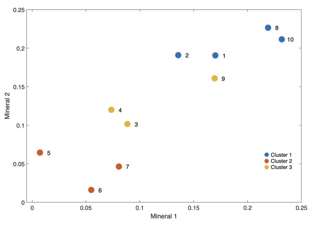
The we perform spectral clustering using spectralcluster. The function partitions the sediment samples in the n-by-p data matrix data into k=3 clusters using the spectral clustering algorithm. The output is the cluster indices of each sediment sample and the eigenvectors of the Laplace matrix.

[idx,V] = spectralcluster(data,3)

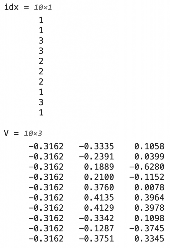
We can display the result visually.

figure('Position',[50 500 600 400])
h5 = gscatter(data(:,1),data(:,2),idx);
hold on
for i = 1 : size(h5,1)
set(h5(i),'Marker','o',...
   'MarkerSize',10,...
   'MarkerFaceColor',colors(i,:))
end
text(data(:,1)+0.005,data(:,2),lbs,...
   'FontSize',10)
xlabel('Mineral 1')
ylabel('Mineral 2')
legend('Cluster 1','Cluster 2',...
   'Cluster 3','Box','Off')
hold off

k-Nearest Neigbors Classification and Clustering

Although the method is often referred to as k-nearest neighbour classification and clustering, strictly speaking it is not clustering, nor is it a method of unsupervised classification. In fact, a training data set with objects and their assignment to groups is used to subsequently assign new objects to these groups using the next neighbor criterion. The advantage of using k nearest neighbours instead of making an assignment based on the known assignment of the one nearest neighbour is obvious: the result is more reliable. Alternatively, we can search for objects that are located within a given distance r and use their known assignment to assign a new object to a group. As an alternative to searching for a specific number k of nearest neighbors, we can search for objects that are located within a given distance r. The same distance measures are used here as for hierarchical clustering, such as the Euclidean distance or cityblock distance. The next neighbor criterion can, however, be used to cluster the data. Clusters are then formed by finding groups of objects with many close neigbors inside the group, but few connections to objects outside. The result corresponds to that of hierarchical clustering if all neighbours of an object are taken into account, i.e. the number is not limited to k. Since the method uses the distance of the nearest neighbors as a measure of this difference, the method is used if there is natural heterogeneity in the data set that cannot be attributed to random noise.

clear, clc, close all
data = load('sediments_4.txt');

We then create decent colors for the graphics.

colors = [
   0      0.4470 0.7410
   0.8500 0.3250 0.0980
   0.9290 0.6940 0.1250
   0.4940 0.1840 0.5560
   0.4660 0.6740 0.1880
   0.3010 0.7450 0.9330
];

We use the 9 samples for the training data set and the nth sample for testing, which in our example is n=9. The returned indices are sorted according to distance. As expected, the listed Euclidean distances and the sorted nearest neigbors agree with the result of hierarchical clustering if we use all nearest neigbors, which is 10, but it’s actually only 9 because we used one for testing.

n = 9;
X = data;
Y = data(n,:);
X(n,:) = NaN;
[idx1,C1] = knnsearch(X,Y,'K',10)

We prepare data, leaving the nth data point out for testing.

X = data;
Y = data(n,:);
X(n,:) = NaN;
ids = (1:10)';
lbs = num2str(ids);

Alternatively, we can search for objects within specific Euclidean distance. We use a radius r=0.012 for the Euclidean distance and assign the testing sample to a group according to the 10 column of data.

[idx1,C1] = rangesearch(X,Y,1.2)

Since we have the expected cluster ID in the 10th column of data, we can actually look up the assignments, in this case the first four IDs are all 1.

data(cell2mat(idx1),10)

The result leads to the expected result, the nth sample is assigned to the correct cluster 1. We can display the result visually using

figure('Position',[50 500 600 400])
h4 = gscatter(X(:,1),X(:,2),X(:,10));
hold on
for i = 1 : size(h4,1)
set(h4(i),'Marker','o',...
   'MarkerSize',10,...
   'MarkerFaceColor',colors(i,:))
end
text(X(:,1)+0.005,X(:,2),lbs,...
   'FontSize',10)
line(Y(:,1),Y(:,2),...
   'Marker','Square',...
   'MarkerSize',10,...
   'MarkerFaceColor',[0 0 0],...
   'Color',[0 0 0],...
   'LineStyle','None')
text(Y(:,1)+0.005,Y(:,2),lbs(n,:),...
   'FontSize',10)
xlabel('Mineral 1')
ylabel('Mineral 2')
legend('Cluster 1','Cluster 2',...
   'Cluster 3','Cluster 4',...
   'New Data Point',...
   'Box','Off')
hold off

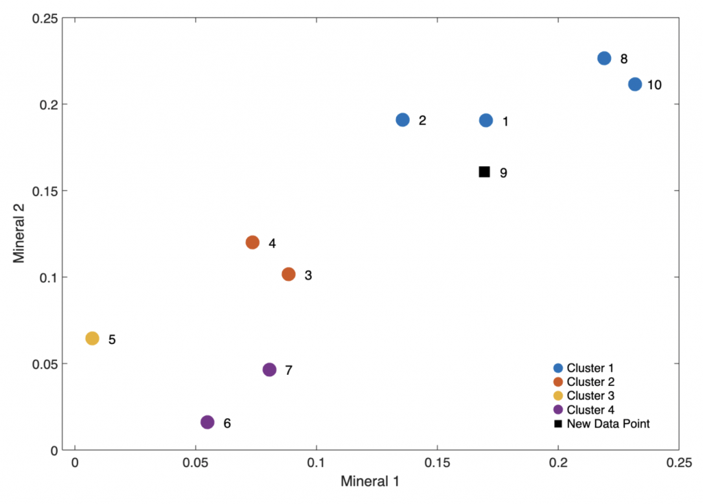
It is also clear that the assignment of the sample with the number 9 is correctly assigned to cluster 1.

Downloads

Download Live Script and Data

References

Hermanns R, Trauth MH, McWilliams M, Strecker MR (2000) Tephrochronologic constraints on temporal distribution of large landslides in NW-Argentina. Journal of Geology 108:35–52.

Kubat M (2017) An Introduction to Machine Learning. Springer, New York Dordrecht Heidelberg London.

Lein JK (2012) Environmental Sensing, Analytical Techniques for Earth Observation. Springer, New York Dordrecht Heidelberg London.

Neuer MJ (2024) Maschinelles Lernen für die Ingenieurwissenschaften, Einführung in physikalisch informierte, erklärbare Lernverfahren für KI in technischen Anwendungen. Springer Vieweg, Berlin.

Petrelli M (2023) Machine Learning for Earth Sciences, Using Python to Solve Geological Problems. Springer Nature, Switzerland.

Pflaumann U, Duprat J, Pujol C, Labeyrie LD (1996) SIMMAX: A modern analog technique to deduce Atlantic sea surface temperatures from planktonic foraminifera in deep-seasediments. Paleoceanography 11:15–35.

Vincens A, Buchet G, Servant M, ECOFIT Mbalang Collaborators (2010) Vegetation response to the “African Humid Period” termination in Central Cameroon (7° N) – new pollen insight from Lake Mbalang. Climate of the Past 6:281–294.