
The journey of NASA’s EO-1 satellite is coming to an end. The images recorded by the Hyperion Sensor, aboard the satellite, during the past years, will provide valuable information about the Earth’s surface for many years to come.
The Earth Observing-1 Mission (EO-1) satellite is part of the New Millennium Program of the US National Aeronautics and Space Administration (NASA) and the US Geological Survey (USGS), which began with the launch of this satellite on 21st November 2000.
EO-1 has two sensors: the Advanced Land Image (ALI) has nine multispectral bands with a 30 m spatial resolution and a panchromatic band with a 10-m resolution, and the hyperspectral sensor (Hyperion) has 220 bands between 430 and 2,400 nm (Mandl et al. 2002, Line 2012). Hyperion data (together with data from of other NASA satellites) are freely available from the USGS Earth Explorer webpage.
The EO-1 User’s Guides provides some useful information on the data formats of these files (Barry 2001, Beck 2003). We can import the data of an image showing Lake Magadi in the southern Kenya rift from the EO1H1690582013197110KF.L1R file using
clear
HYP = hdfread('EO1H1680612008182110KF.L1R',...
    '/EO1H1680612008182110KF.L1R', ...
    'Index', {[1 1 1],[1 1 1],[3189 242 256]});
We need to permute the array to move the bands to the third dimension by typing
HYP = permute(HYP,[1 3 2]);
The radiance for the shortwave infrared (SWIR) bands (bands 71 to 242) is calculated by dividing HYP by 80:
HYPR(:,:,1:70) = HYP(:,:,1:70)/40;
HYPR(:,:,71:242) = HYP(:,:,71:242)/80;
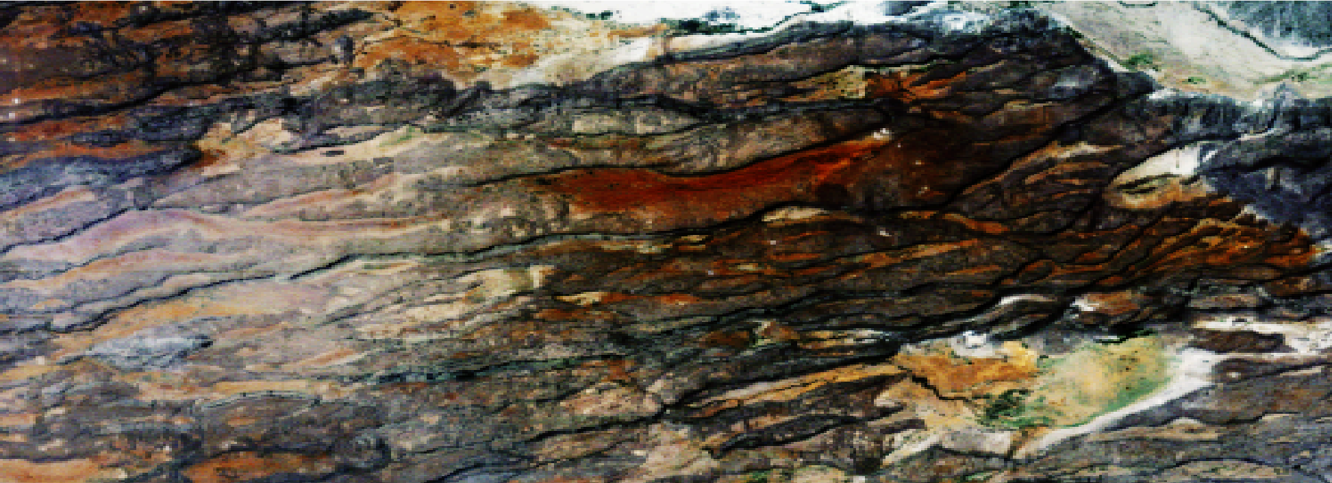
In order to create an RGB composite of bands 29, 23 and 16, we can extract the bands from the radiance values data HYPR by typing
HYP1 = HYPR(:,:,29);
HYP2 = HYPR(:,:,23);
HYP3 = HYPR(:,:,16);
Since most of our radiance values are within the range [0,255], we use uint8 to convert our data to the uint8 data type without losing much information.
HYP1 = uint8(HYP1);
HYP2 = uint8(HYP2);
HYP3 = uint8(HYP3);
We then use histeq to enhance the contrast in the image and concatenate the three bands to a 3,189-by-242-by-3 array
HYP1 = histeq(HYP1);
HYP2 = histeq(HYP2);
HYP3 = histeq(HYP3);
HYPC = cat(3,HYP1,HYP2,HYP3);
and display and save the result by typing
imshow(HYPC), axis off
print -dtiff -r1200 magadi.tif
You find more details about processing Hyperion images with MATLAB in the MRES book.
References
Barry P (2001) EO-1/Hyperion Science Data User’s Guide. TRW Space, Defense & Information Systems, Redondo Beach, CA
Beck R (2003) EO-1 User Guide. USGS Earth Resources Observation Systems Data Center (EDC), Sioux Falls, SD